How to make a mesh dance in real time to music
Live demo · Source · The drum problem
Driving a mesh with sound
Take the natural vibration modes of a 3D shape, its manifold harmonics, and drive them with the frequency content of live audio. Arbitrary meshes “dance” to arbitrary music in real time, in a browser, with no install. There are some preloaded meshes and songs.
Pick a mesh (a sphere, a torus, a plane, or a few real scanned busts), pick an audio source, press
play, and watch the mesh dancing :) You can also drop in your own .obj, .ply, .stl or .glb,
which gets welded, decimated and eigen-solved live in a Web Worker. Uploading triggers a real
eigensolve, so expect a couple of seconds depending on vertex count. The built-in meshes were solved
ahead of time and load instantly.
Drive and intensity scale how hard the mesh is pushed, modes sets how many harmonics are active (a level-of-detail knob), smoothing sets how quickly a mode settles, and inspect freezes the audio and oscillates one eigenmode so you can see a single standing wave.
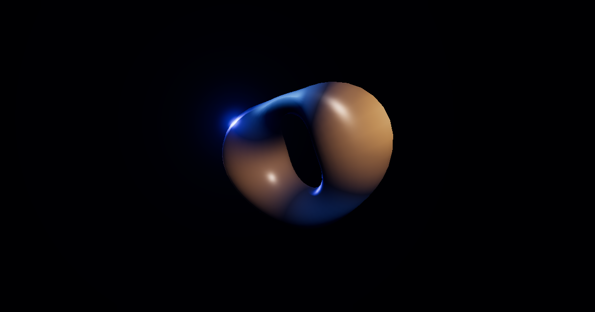
Manifold harmonics?
Audio transforms into a frequency space, where filtering becomes easy. The nice surprise is that meshes have a frequency space too.
Take a drum head. Hit it and it doesn’t wobble arbitrarily; it rings in a discrete set of standing waves whose shapes are determined entirely by the drum’s geometry. Mark Kac asked in 1966 whether you could run that backwards: can one hear the shape of a drum?
On a triangle mesh those standing waves are the eigenvectors of the discrete Laplacian, its manifold harmonics. Low eigenvalues are slow global wobbles, high eigenvalues fine ripples: the same low-to-high ordering an FFT gives you, over a surface instead of over time.
With this you can let the song drive the shape and get Kac’s question the other way. instead of hearing a shape, you see a sound.
How does it work?
1. Build the Laplacian
Cotangent weight per edge: w_ij = ½(cot α + cot β), where α and β are the angles opposite edge (i,j) in the two triangles sharing it. Off-diagonal L_ij = −w_ij, diagonal L_ii = Σ_j w_ij. The mass matrix M is diagonal, with M_ii one third of the area of the incident triangles; this is what makes the operator depend on geometry rather than connectivity alone. Both are stored sparse (CSR).
2. Solve for the lowest modes
Solve L φ = λ M φ, rewritten in symmetric standard form A y = λ y with A = M^(−1/2) L M^(−1/2).
The full basis is an n×n eigendecomposition, O(n³). Only the lowest 24 modes are needed, so the solver uses block LOBPCG, which requires nothing beyond sparse matrix–vector products. It deflates the constant λ=0 mode, oversamples with guard modes, warm-starts with weighted-Jacobi sweeps to damp high-frequency content in the random initial guess, and stops once the eigenvalues stabilise.
3. Band the audio
One AnalyserNode taps the active source (synth, loop, microphone, file, or YouTube). Its FFT is
reduced to K log-spaced bands from 40 Hz to 12 kHz, each normalised from a −90…−25 dB window into
[0,1]. Log spacing gives equal musical intervals per band; linear bins would put most of them above
6 kHz.
4. Band k drives mode k
Both spectra are ordered low to high, so bass drives the global modes and treble the fine ones. Each amplitude has a 40 ms attack and a 280 ms release.
5. Displace along the normals
Each vertex moves along its rest-pose normal by the weighted sum of the modes:
p_i = base_i + normal_i · ( Σ_k amp_k · φ_k(i) ) · intensity
The displacement is additive: the rest shape is preserved and vibrated, not reconstructed from filtered coordinates, so the mesh stays recognisable at any drive level.
Steps 1 and 2 run once per mesh. Steps 3, 4 and 5 run every frame.
Also see
- Vallet & Lévy, Spectral Geometry Processing with Manifold Harmonics, Eurographics 2008. The manifold-harmonics formulation, including the symmetrisation used here.
- Meyer, Desbrun, Schröder & Barr, Discrete Differential-Geometry Operators for Triangulated 2-Manifolds, 2003. The cotangent weights and lumped mass matrix.
- Knyazev, Toward the Optimal Preconditioned Eigensolver: LOBPCG, SIAM J. Sci. Comput. 2001.
- Kac, Can One Hear the Shape of a Drum?, Amer. Math. Monthly 73, 1966. The answer is sort of no! Gordon, Webb and Wolpert built two different drums with identical spectra in 1992.
- A very similar thing but from 2011: ManifoldMusic from TU Wien’s Visualisierung 2 course (2013) did the same audio-drives-manifold-harmonics idea as a desktop application, computing the full basis and filtering the coordinates, and hit that O(n³) wall at about a minute of load time per mesh.
see the code: github.com/HughParry/music-mesh-transforms